Recursive Zero-Knowledge Proofs: A Comprehensive Primer
Posted
Recently, there have been a number of exciting results concerning proof recursion. A sketch for Halo has suggested the possibility of proof recursion without a costly trusted setup, while Fractal has demonstrated the first instantiation of proof composition which is post-quantum secure. We’ll go into these results later after discussion what proof composition is, the technical challenges associated with achieving it, and how it ties into commonly used proof systems as Groth 16 and Bulletproofs.
There are a number of use cases for recursive composition. One of the most well-known at the moment is that of Coda, a fully-succinct blockchain protocol allowing clients to validate the entire chain by checking a small cryptographic proof in the tens of kilobytes. Recursive proofs have also been proposed for other blockchain scaling solutions, such as recursively proving validity of Bitcoin’s proof of work consensus algorithm, and at Celo using bounded recursion to efficiently verify aggregated signatures for mobile clients.
A use case outside of the blockchain space concerns proving legitimacy of photographs. You could, for example, prove that an original photograph was modified only with crop and rotation operations. Each update of the photo would require one additional layer of proof recursion, updating $\pi_{n-1}$ attesting to the last $n-1$ photo operations being legitimate, to a proof $\pi_n$ of the exact same size attesting to the last $n$ operations.
This post has two intentions; to serve as an introduction to recursive proof composition and the technical challenges which arise in achieving it, and also as a crash-course in the computational model most commonly used for zero-knowledge proofs; that of arithmetic circuits. As we will see, the first goal cannot be realized without the second. The challenges involved in constructing recursive proofs involve many fundamental aspects of circuit construction encountered in practice, such as the connection between the choice of elliptic curve and arithmetic circuit used, in addition to the impact of the structure of a circuit’s input and the use of hash functions. While we will be giving a theoretical exposition, every piece of it will be relevant in practice for the engineering of general-purpose zero-knowledge proofs.
As such, this post is suitable for anyone who either has worked with ZKPs before and wants to know how recursive proofs work, or for anyone wanting to learn at an introductory level how arbitrary ZKPs are engineered in practice given an existing proof system.
Most of the discussion will be at a relatively high and intuitive level; it is assumed only that the reader has a basic familiarity with zero-knowledge proof systems, group theory, and computational complexity up to understanding the class of problems known as NP.
We also alternate between additive and multiplicative notation where each is most intuitive, sacrificing consistency for the sake of clear exposition. Multiplicative notation $g^ah^b$ is used when considering details relevant to any group, while additive notation $[a]P + [b]S$ is used when considering details specific to elliptic curve groups, or specific enough to justify its use.
We will begin with a brief review of proof systems and arithmetic circuits.
General-Purpose Proof Systems
A zero-knowledge proof system consists of a prover $P$ and a verifier $V$. Given some public input $x$ and private witness $w$, the prover produces a proof $\pi$. The verifier then takes in the public input $x$ and proof $\pi$ and outputs 1 if the proof is correct, 0 if it is not. This is done without the verifier learning $w$.
$\textbf{Note}$: Technically in practice we use argument systems rather than proof systems proper. In an argument system, the prover is too computationally bounded to “trick” the verifier into accepting a fake proof. In some sense it is a rigorous formulation of the principle that you can trust someone more if they have fewer resources to use against you. We will abuse terminology here by referring to argument systems as proof systems, as the language is mildly more intuitive.
NP is the class of “efficiently” verifiable problems, or of problems which can be verified in polynomial time. In other words, $L \in NP$ if there is some polynomial-time verifier $V$ analogous to the verifier discussed above such that for every $x \in L$, there exists some witness $w$ such that $V(x,w) = 1$. In the context of proof systems, we will become used to thinking of $x$ in terms of public input, and $w$ in terms of private input. We will also take the NP-relation $R$ as a description of the verifier’s output, so that $V(x,w) = R(x,w)$ on all inputs $(x,w)$; the difference is that $V$ is an algorithm with time and space complexity, whereas $R$ abstractly maps to the correct answer.
We will again abuse terminology in this post by referring to $w$ as “private” input. While it will be hidden from the verifier if using a zero-knowledge proof system, we can also instantiate recursive proofs with a system that does not provide zero-knowledge, and thus does not hide $w$ from the verifier. This is justified by the fact that in either case the verifier does not take in $w$ as input.
Given the symmetry of our two definitions of verifiers above, we might guess that proof systems are particularly useful for NP relations. This is in fact true, particularly since we can construct them for NP-complete problems. An NP-complete problem is one which is in NP and for which any NP problem can be reduced to it. In practice this means that is it efficiently verifiable and that we can both in theory and in software build a compiler which reduces any NP problem to it.
As a brief example, 3-colorability is NP-complete, and we can build zero-knowledge proof systems for it. In theory we could build a compiler such that for any program in our specified format expressing an NP relation, we can compile it down to an equivalent problem expressed in terms of 3-colorability. In practice this would be very inefficient.
We would like a more natural computational model for proof systems. We can think of modern computer architecture as being based on performing bit operations. This raises a question; what fundamental operations would we like our new model based on some NP-complete problem to use? Much of modern public-key cryptography including proof systems uses elliptic curve groups, or points $(x,y)$ in some field $\mathbb{F}$ where $x,y \in \mathbb{F}$ and satisfy a particular equation, such as $y^2 = x^3 + 5$. Examples of fields are the real numbers $\mathbb{R}$, the complex numbers $\mathbb{C}$, and finite fields $\mathbb{F}_q$. In cryptography we often work with large finite fields, which effectively just use addition and multiplication taken mod $q$. We can then define an abelian group operation $\cdot$ complete with identity, inverses, associativity, and commutativity on these points such that $(x,y) \cdot (x’,y’) = (x”, y”)$ where all 3 points lie on our particular choice of curve over our base field $\mathbb{F}$.
There is a crucial point to understand here. Suppose we have an elliptic curve $G$ defined over a base field $\mathbb{F}_q$, such that the order of $G$ is $r$, or $|G| = r$. This tells us elements of the group will “cycle back” after $r$ operations, so that if $g \in G$ then $g^r = 1$ the identity (also known as $O$ the point at infinity for elliptic curves in particular). This means if we have $g^x$, $g \in G$ implies $x \in \mathbb{F}_r$. Taking the Bulletproofs argument system as an example, the prover’s secret input is expressed as 3 vectors $\textbf{a_L}, \textbf{a_R}, \textbf{a_O} \in \mathbb{F}^n_r$. The prover’s first two computations are
where also $\alpha, \beta \in \mathbb{F}_r$, $h \in G$, and vectors $\textbf{g}, \textbf{h} \in G^n$. This exponentiation, here performed element-wise using vectors, is referred to as scalar multiplication using elliptic curves. The field $\mathbb{F}_r$ is known as the scalar field of the curve. Notice what we have done in these two lines of computation; in order to represent our problem and its inputs as multiples of elliptic curve group elements, we want to translate its inputs and constraints to be in the field $\mathbb{F}_r$ where $|G| = r$. But note that $\mathbb{F}_r$ is $\textbf{not}$ the base field $\mathbb{F}_q$ that $G$ is defined over. Here we are abstracting over the details of the group operation, but its concrete implementation will use arithmetic mod $q$, as for $(x,y) \in G$ we will be operating on points $x,y \in \mathbb{F}_q$. This will become very important in our later discussion of recursive composition, as at first glance we will need to represent elliptic curve operations performed in $\mathbb{F}_q$ in terms of $\mathbb{F}_r$ elements.
Given that we want to express our inputs in the field $\mathbb{F}_r$ which is equal in size to our elliptic curve group $G$, there is a natural computational model we can use, that of arithmetic circuits. An arithmetic circuit is simply a circuit defined over some field $\mathbb{F}$ such that each gate performs addition or multiplication on its inputs.
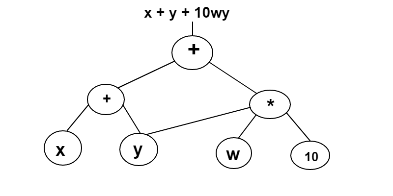
The NP-complete problem we want to target for our proof system is thus arithmetic circuit satisfiability. Intuitively we can think of this as an NP-relation $R$ such that for every circuit $C$, there is some satisfying input $w$ consisting of elements in $\mathbb{F}$ such that $R(C,w)$ = 1, or $C(w) = 1$.
$\textbf{Note}$: It is worth mentioning here that not all general proof systems reduce the relation they are using down to an NP-complete problem, but broader classes of problems such as NEXP as done by AIR, effectively an algebraic representation of a computation with polynomially bounded space; this is used by STARKs. Such representations allow program descriptions to shrink relative to their actual size, similar to how a while loop executed 10 times provides a 10x reduction in program description. In the case of NP reductions, space and time complexity are equivalent, so that a computation repeated 10 times will increase the size of the description of the program or circuit by 10x. This is the case we will consider here, as it is where the most success has been found in achieving recursive composition of proofs.
Earlier we mentioned compiling NP problems down to our single NP-complete problem so thart we can use a single proof system for any NP relation. But there is a very subtle point here which can be a bit confusing. Let $R$ be the NP relation for arithmetic circuit satisfiability discussed above, and say we have a relation $R’$ that takes in public input $x$ your name and private input $w$ your credit card number. We can then express $R’$ in terms of arithmetic circuit satisfiability, such that both $x$ and $w$ are expressed in terms of elements of $\mathbb{F}$. However, $R’$ here is not $R$. $R’$ is a specific instance of arithmetic circuit satisfiability such that both $x$ and $w$ are inputs to a fixed circuit, rather than $x$ itself being the circuit. This can be a confusing point of notation coming from computational complexity to zero-knowledge proof systems.
Bit Operations
We will continue by outlining a proof that arithmetic circuit satisfiability is NP-complete, and in doing so will uncover some practical considerations when constructing arithmetic circuits in practice; these will be particularly relevant later when discussing a technical difficulty involving hashing inside of a circuit in our recursive proofs construction.
Recall that to show a problem is NP-complete, we can simply reduce another NP-complete problem down to it. This implies we can reduce any problem in NP down to the one we are considering.
Boolean circuits, while less practical for general-purpose zero-knowledge proofs, are more widely studied in computational complexity theory than their arithmetic counterparts. They are like arithmetic circuits described above, except that each gate computes one of boolean operations AND, OR or NOT on its inputs (or some equivalent set of operations; using only NAND is equally expressive). In fact, the canonical example of an NP-complete problem, 3-SAT or satisfaction of boolean formulas with clauses of at most size 3, can easily be reduced to boolean circuit satisfiability. Simply make each variable an input to the circuit, and each operation in the formula a gate.
To reduce boolean circuit satisfiability to arithmetic circuit satisfiability is slightly harder but still fairly simple. Every boolean operation can be effectively simulated by field element operations. In particular, suppose we want to “unpack” a field element $x \in \mathbb{F}_p$ into a bit representation $b_1b_1…b_n$. Then for each bit $1 \leq i \leq n$ we check that
in addition to checking that
This is assuming we do not care about the summation on the left being larger than the modulus, which we would in practice. This check would take just over another n constraints.
To simulate AND for two $\mathbb{F}_p$ elements $x,y$ with representations $b_1…b_n$ and $b_1’…b_n’$ respectively, and with $x$ AND $y$ = $z$ where $z$ has representation $b_1…b_n”$, we add the constraint $b_i \times b_i’ = b_i”$ for each $1 \leq i \leq n$. Similarly, for OR we add the constraint $b_i \times (b_i - b_i’) = b_i” - b_i’$, and for NOT on a single bit the constraint $(-1 \times b_i) + 1 = b_i”$. It’s easy to verify that each of the four inputs $(0,0)$, $(1,0)$, $(0,1)$ and $(1,1)$ check out in each case.
Notice that we have performed here a sleight of hand. We have not explicitly constructed a circuit but rather a list of constraints which may be expressed in circuit form. In fact, many modern proof systems use directly so-called “R1CS” or Rank-1 Constraint Systems such as the one shown above, both in theory and in software compilers meant for users to encode NP relations. R1CS is another NP-complete problem similar in form to arithmetic circuit satisfiability as only operations over a fixed field are used. Systems such at Groth16 take the additional intermediate step of compiling the R1CS down to what is known as a Quadratic Arithmetic Program, or QAP, an NP-complete problem having to do with the satisfaction of certain kinds of polynomials. Still other systems such as the newer PLONK or Sonic eschew R1CS altogether in favor of using the satisfaction of other certain kinds of polynomials for their schemes. This justifies the use of arithmetic circuit satisfiability both here and in the literature as an abstraction that subsumes all constraint systems used in practice, as the simplest and most intuitive way of thinking about the computation of any NP problem using only field additions and multiplications.
We’ve effectively shown that arithmetic circuit satisfiability is NP-complete by reducing boolean circuit satisfiability down to it. But how well can we perform boolean operations inside arithmetic circuits in practice? Many useful algorithms operate on bit values. In the current most well-known and used proof systems such as Groth16 and Bulletproofs, addition gates are “free” while multiplication gates cost 1. In fact, the secret inputs to Bulletproofs $\textbf{a_L}, \textbf{a_R}, \textbf{a_O}$ mentioned above act as vectors of the left inputs, right inputs, and single outputs of each multiplication gate; the circuit itself is compiled down to a set of linear constraints (typically in practice this is constructed directly, bypassing the circuit representation altogether; these models are similar enough that intuitions from one will carry over to the other). By the above construction, simply representing a field element in terms of bits causes a logarithmic blowup in complexity by adding one multiplication per bit.
Throughout this post we will make use of SNARKs in which the prover’s memory and time complexity both increase linearly or worse with the cost or number of multiplication gates in our circuit. This can make very large circuits painful to work with.
The asymmetry above between field operations and bit operations means that while $x \times y = z$ costs 1 constraint, computing $x$ AND $y$ = $z$ costs $O(log_2(p))$ constraints; on the order of $log_2(p)$ for both unpacking $x$ and $y$ into bits and to add the constraints for the AND operation, in addition to 1 additional constraint for packing the result $z$ with $(\sum b_i” 2^{i-1}) \times 1 = z$. Since the size of the modulus $p$ we use for the field of our circuit, or equivalently the size of the elliptic curve group we use, can be quite large, this can be a massive cost; typically the number of bits $log_2(p)$ is at least 256. This will matter greatly when considering the hash function used to instantiate recursion later in the post.
Proof Recursion
Recall that in a general purpose proof system, a prover creates a proof $\pi$ that it knows some satisfying public input $x$ and private input $w$ to some NP-relation $R$ specified by an arithmetic circuit, i.e. $\pi$ attests to the fact that $R(x,w) = 1$. A verifier will then take in the produced proof $\pi$ and public input $x$, and output 1 if the proof is valid. But this verification itself can be expressed as an NP-relation $R’$, so that $R’(x, \pi) = V(x, \pi)$ for all valid inputs to the verifier. Thus, we can create proofs which attest to the validity of other proofs.
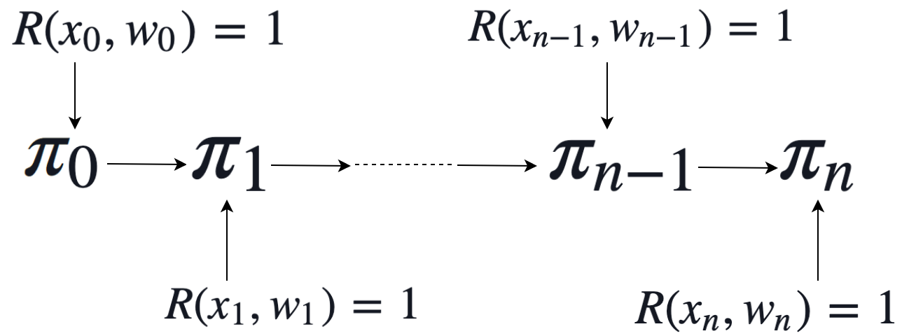
In the simplest case our recursive proofs will prove a relation $R$ inductively. In other words, we will have a “base” proof $\pi_0$ which attests to the prover knowing some input $(x_0,w_0)$ such that $R(x_0,w_0) = 1$. The proof $\pi_n$ for any $n > 0$ will then prove that the prover knows $(x_n, w_n)$ such that $R(x_n, w_n) = 1$ and that a proof $\pi_{n-1}$ was produced attesting to the knowledge of $(x_{n-1}, w_{n-1})$
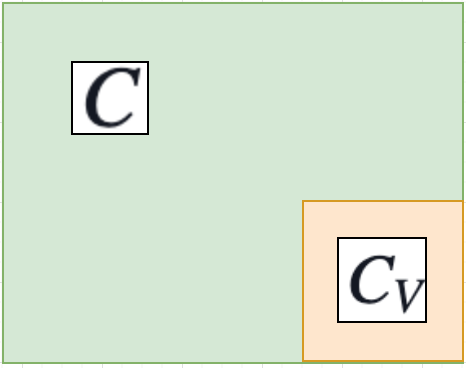
How could we do this? First we would build a circuit $C_V$ for our verifier $V$. We would then build a circuit $C$ which would either verify $R(x_0,w_0) = 1$ (for the base case) or verify $R(x_i,w_i) = 1$ and then check $V(x_i, \pi_{i-1}) = 1$.
In practice this raises several questions. What exactly does the input to our circuit look like? Does our choice of elliptic curve, and equivalently our choice of field the circuit is defined over, matter? How does the verifier encoded in our circuit know what NP-relation $R$ it is evaluating? We will answer these questions over this and the next two sections, starting with the last.
A preprocessing SNARK $(G,P,V)$ such as Groth16, Marlin, or PLONK has an additional generator algorithm $G$ which produces a proving key $pk$ and verifier key $vk$ given a description of the program being used. We can think of these keys as smaller summaries of the circuit we are using which can replace the program description as input to the prover and verifier respectively. Without some reasonably short summary of $C$, it would appear that we need to pass a description of $C$ into $C$ itself, which would be costly. By taking as input the verification key $vk$, the verifier already has sufficient knowledge of the structure of $C$. This, in addition to the relative efficiency their constructions have achieved, motivates our use of a preprocessing SNARK.
To determine what we will want our input $(x,w)$ to look like, it will help to examine an abstraction known as proof-carrying data. Effectively it is just a prover algorithm $\mathbb{P}$ and a verifier algorithm $\mathbb{V}$ such that they are designed to create and verify proofs for a distributed, trustless computation. Using a PCD, I can compute some function $F$ with output $y$, pass you $y$ in addition to a proof $\pi$ that it was computed correctly, and you can then compute $y’ = F(y)$ with proof $\pi’$, and then pass both onto someone else. More generally, given a PCD $(\mathbb{G}, \mathbb{P}, \mathbb{V})$, we can prove the correct iterated computation of a function $F$ such that
where each iteration of $F$ is computed by a different party, none of whom are trusted. In other words, we prove $y_i$ is the result of iterating $F$ on $x$ a total number of $i$ times. This is exactly the problem we are solving by creating inductive chains of proofs, with the exception that we also allow for some distinct “local” private data $w_i$ at each iteration. $F$ could be, for two examples, either the addition of a block to a blockchain, or the application of a rotation operation to a digital photograph.
A bit more precisely, we can say that we have a list of input tuples $(x_1, w_1), …, (x_n, w_n)$ such that, for example, $x_4 = F(F(F(x_1, w_1), w_2), w_3)$.
What do the inputs to a PCD look like? We will allow our notation here to become slightly confused in order to agree with the literature, noting where our PCD notation is analogous to the notation used earlier in our discussion of proof systems.
After the proving and verification keys $(pk, vk)$ have been generated by $\mathbb{G}$ with a single initial setup, the prover $\mathbb{P}$ will take in $pk$, an input message $z_{in}$, a proof $\pi_{in}$, some local data $z_{loc}$, and the claimed result of the computation $z$. If we are computing the $n$-th proof $\pi_n$, then $z_{in}$ will be the output generated when computing the $(n-1)$-th proof $\pi_{in} = \pi_{n-1}$. The local data $z_{loc}$ is effectively our $n$-th private witness $w_n$ which only the prover has access to, whereas the claimed output $z$ is analogous to the $n$-th public input $x_n$. Note that $z = x_n$ can be both the claimed output of some computation $F$ while still being the input to a proving system.
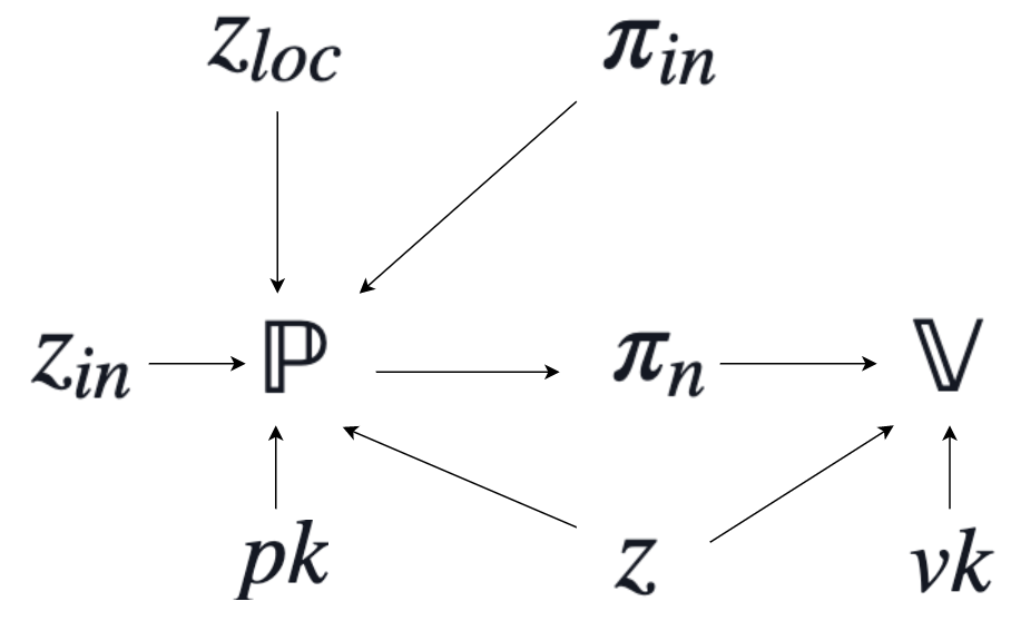
The verifier $\mathbb{V}$ takes in fewer inputs; $vk$, the claimed result $z$, and the prover generated proof $\pi_n$ attesting that $z$ is correct. The proof in fact attests that $z$ satisfies a fixed compliance predicate $\Pi$ which is effectively the NP-relation $R$ discussed earlier, or the application of our transition function $F$. $\Pi$ takes as input $z$ ,$z_{loc}$, $z_{in}$, in addition to a bit $b_{base}$ indicating whether we are dealing with inputs to our original base case. Note that $\Pi$ does not take proofs as input; it will rather be used as a sub-circuit in the process of proof creation.
Above we have a diagram illustrating the PCD construction when generating proof $\pi_n$. Note that at the next step when generating $\pi_{n+1}$, we will have $\pi_{in} = \pi_n$, and $z_{in} = z$ where $z$ and $\pi_n$ were both used in step $n$.
We are now able to give a preliminary answer to what our public input $x$ and private input $w$ should be. Recall that the verifier and prover both have access to $x$, while only the prover has access to $w$. Recall also that in our PCD outline the only input the verifier needs access to is $z$, the claimed output at our current step of recursive composition. In addition, since we will encode the verifier $V$ in the circuit, both the prover $P$ and the verifier $V$ will need access to the verification key $vk$. Thus, we can set $x = (vk, z)$ and $w = (z_{loc}, z_{in}, \pi_{in})$. This turns out not to work in practice, and we will proceed to complicate it in two ways. First, by needing two circuits defined by two distinct elliptic curves which in turn instantiate two different verifiers, yielding two different verification keys. Second, by using hashing inside of one of these two circuits in order to reduce the size of the verification keys.
There is one extension that can be made to the above PCD scheme. We have been discussing an inductive chain of proofs, and will continue to assume we are working in the case for most of the rest of this post. However, we can also extend $\pi_{in}$ and $z_{in}$ to vectors of inputs rather than single inputs. This allows us to create trees of proofs, and will become important later when discussing some theoretical issues that arise in proving the security of unbounded proof recursion.
On top of this discussion we should be careful to emphasize that as far as we are concerned for proof recursion there is no additional “special” machinery specific to constructing PCDs; it is simply an abstraction used to define what it is to perform computations securely in a trustless and distributed manner. For our purposes here it is less an object in its own right and more of a rigorous outline of what we hope to achieve in practice through recursive proofs.
Cycles of Elliptic Curves
We will now discuss the most important practical constraint encountered when working to achieve proof composition; the choice of elliptic curve used to instantiate our system. The most efficient and useful SNARKs use pairings in their construction. To make use of them we will need to choose a pairing-friendly curve. This requirement significantly constrains our choices of elliptic curves. And in fact, we will need not one but two.
Recall that we want to choose an elliptic curve $G$ over some base field $\mathbb{F}_q$. This curve will have some size $|G| = r$ which will be the size of the curve’s scalar field $\mathbb{F}_r$ which we also want to use to instantiate our arithmetic circuit. In particular, this means that we will naturally perform $\mathbb{F}_r$ operations inside of our circuit, but when computing operations on elliptic curve points inside of our proof system verifier we will be performing $\mathbb{F}_q$ operations. This normally would not be an issue, but here we are encoding our verifier inside of our arithmetic circuit; thus, we will need to simulate $\mathbb{F}_q$ arithmetic inside of $\mathbb{F}_r$ arithmetic. This might be confusing, but it’s very important; take a moment to think about it if you need to.
The obvious solution is to choose some curve such that $q = r$. This is not possible, as we know from theory that $r$ will divide $q^k - 1$ where $k$ is our curve’s embedding degree thus $r \not= q$. The next clear idea is to simulate $\mathbb{F}_q$ arithmetic using $\mathbb{F}_r$ arithmetic. This means, however, that we will need to take $F_q$ elements mod $r$ to deal with overflow, which in particular requires bit operations. As we discussed above in our proof sketch that arithmetic circuit satisfiability is NP-complete, this leads to a logarithmic blowup in complexity in the size of the circuit field $\mathbb{F}_r$, or by a multiplicative factor of the number of bits of the field. At first glance this gives us an increase in circuit size by a factor of at least 256, which is pretty massive. There is not much that can be done to improve this approach.
There is, fortunately, a better option. The intuition is that we want to construct two circuits so that we can cycle back and forth between them, getting the verifier and circuit arithmetic to always be over the same field.
Suppose we have two elliptic curves $G_r$ and $G_q$ defined over $\mathbb{F}_q$ and $\mathbb{F}_r$ respectively. Then we create two circuits $C_r$ and $C_q$, one for each curve, and also instantiate preprocessing SNARKs $(G_r, P_r, V_r)$ and $(G_q, P_q, V_q)$ with each curve respectively. We run generator $G_r$ on circuit $C_r$ to obtain key pair $(pk_r, vk_r)$, and we run generator $G_q$ on circuit $C_q$ to obtain key pair $(pk_q, vk_q)$.
How can we use two circuits to acheive one layer of proof recursion? Suppose circuit $C_r$ encodes our compliance predicate $\Pi$ as a sub-circuit, i.e. it checks the correctness of our predetermined NP relation $R$. When the prover $P_r$ runs, it will generate a proof $\pi_r$ attesting that the correct input has been provided to this circuit, including the satisfaction of our compliance predicate $\Pi$ on inputs $z$, $z_{loc}$, $z_{in}$, $b_{base}$. Then, our second “wrapper” circuit $C_q$ can be run to take as input $\pi_r$. The prover $P_q$ can then use this circuit to generate a new proof $\pi_q = \pi_{n+1}$ attesting to the fact that $\pi_r$ is a valid proof, which can then be verified in our “main” circuit at the start of our next $(n+1)$-th layer of recursion.
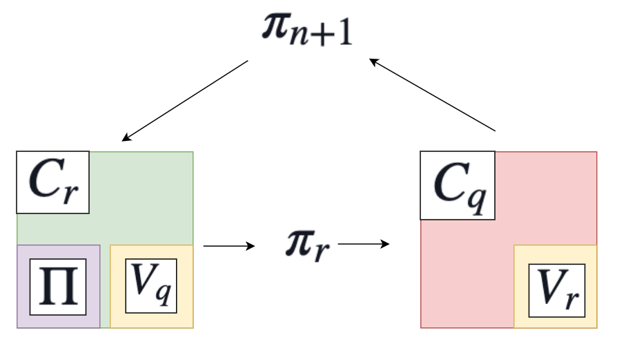
Because the proof $\pi_r$ produced by $P_r$ will be verified in $C_q$, this means that we will need to encode verifier $V_r$ in $C_q$. Similarly, we will need to encode verifier $V_q$ inside of $C_r$. In addition, each verifier will need to be passed the public input of the other circuit; i.e. we will need access to $x_q$ inside $C_r$ and $x_r$ inside $C_q$, suggesting we will need to make our public input $x$ identical between both circuits. We will thus need to call $V_q(vk_q, x, \pi_q)$ inside of $C_r$ and $V_r(vk_r, x, \pi_r)$ inside $C_q$. In pseudocode, $C_r(x,w) = C_r((vk_r, vk_q, z), (z_{loc}, z_{in}, \pi_{in}))$ will perform:
- If $\pi_{in} = 0$, set $b_{base} = 1$, else $b_{base} = 0$
- If $b_{base} = 0$ check that $V_q(vk_q, x, \pi_{in})$ accepts
- Check that $\Pi(z, z_{loc}, z_{in}, b_{base})$ accepts
$C_q(x,w) = C_q((vk_r, vk_q, z), (\pi_q))$ will be simpler:
- Check that $V_r(vk_r, x, \pi_q)$ accepts
Recall that we want to use two elliptic curves $G_r$, $G_q$ such that $|G_r| = r$ is defined over $\mathbb{F}_q$ and $|G_q| = q$ is defined over $\mathbb{F}_r$. We call such curves a 2-cycle. We also require each to support the computation of pairings How can we find such curves?
The MNT Curve Cycles
We will first explain an important property for the security of pairing-friendly elliptic curves, that of a curve’s embedding degree. A pairing function $e$ is typically constructed as a function
where $G_1, G_2$ are disjoint order $r$ subgroups of the $r$-torsion group
where $[r]P$ represents $P$ added to itself $r$ times, and $O$ is the identity or point at infinity. This is the group $E(\bar{\mathbb{F}_q})$, where $\bar{\mathbb{F}_q}$ is the algebraic closure of $\mathbb{F}_q$. The algebraic closure of a field is simply the field, along with all solutions of polynomials with coefficients in that field.
$\mathbb{F}_T^\times$ above simply refers to the multiplicative group of some finite field $\mathbb{F}_T$, or $\mathbb{F}_T$ restricted to multiplication operations. It is also required to be of size $r$.
This might seem complicated, but in fact we obtain all distinct $r+1$ subgroups of the $r$-torsion group by defining a curve over a field extension $\mathbb{F}_{q^k}$ of size $q^k$, where $k$ is the embedding degree of our elliptic curve $G = E(\mathbb{F}_q)$. In other words, $E[r] = E(\mathbb{F_{q^k}})$. For our purposes we can think of the target group as the field extension of order $q^k$, so that the result of our pairing is $G_T = \mathbb{F}_{q^k}$. Numerically, this can be represented by lists of $k$ points in $\mathbb{F}_q$; there are many excellent resources available if further depth is desired, but this is all we will need to know about pairings here.
The fundamental problem in elliptic curve cryptography is the discrete logarithm problem. Given $g,h$, compute $x$ such that $g^x = h$. It is known that this is very difficult to do for apprpriate choices of group. Elliptic curves are used in part because the best attacks against them are slower than for something relying on number factoring, which allows us to use relatively small base fields, which in turn reduces key size.
Using a curve with an efficient pairing function introduces a new potential security flaw. While we can use it to efficiently map curve points to $\mathbb{F}_{q^k}$, an attacker can as well. This means that an adversary can reduce the security of our system also to the discrete log problem of $\mathbb{F}_{q^k}$. In particular, we will be vulerable to attacks if $q^k$ is too small relative to the computational resources available to our attacker.
This means that we want both $q$ and $k$ to be large. But increasing $q$ reduces efficiency of our proof system in two ways, as in our circuits bit operations cost $log_2(q)$ asymptotically, and we need to perform arithmetic mod $q$ in our circuit-encoded verifier. This increases prover time and memory costs. Ideally then we will want curves with high embedding degrees; $k = 12$ is typically regarded as good.
This brings us to some unfortunate news; the only curve cycles found so far are instantiations of the so-called MNT curves. It can be shown that each MNT4 curve of embedding degree 4 has a corresponding MNT6 curve of degree 6. Worse, security reduces to the weaker curve, here MNT4. This means we need a relatively large base field to achieve acceptable levels of security, at nearly 800 bits.
This is not a hopeless situation; several techniques so far have been proposed to get around this limitation. In addition, it is still possible that a better cycle of curves can be found. However, several impossibility results have been found, suggesting that this will be difficult. We will close this section by listing some of them, to give a sense of what the current siutation is like.
Any cycle of MNT curves must alternate between embedding degrees 4 and 6
Cycles using curves of non-prime order do not exist
Cycles using Barreto-Naehrig or Freeman curves, which are known to be of prime order, do not exist
In particular, it is at least possible that useful cycles will be possible for new constructions of prime-order curves, or that they can be constructed using a combination of MNT, BN, and Freeman curves in one cycle together.
Shortening the Message Length
There is a critical problem with the above circuit designs. An arithmetic circuit $C$ takes in a finite number $n$ of field elements as input. We can pass in fewer than $n$ elements, but we cannot pass in more; $n$ here is an upper bound on the input size. An unbounded circuit here makes as much sense as an unbounded physical circuit. Recall that our key pair $(pk, vk)$ is effectively a relatively short description of the structure of $C$ which our prover or verifier need access to. The verifier in particular requires knowledge of that part of the circuit dealing with its public input $x$. However, this means that the size of $vk$ will in part be a function of the size of $x$. In particular $vk$ will always be larger than $x$. However, the verifier does not need to know the private witness $w$. This means that we can successfully encode $vk$ inside of the witness $w$ instead of inside the public input $x$.
Since our design has two verifier keys $(vk_q, vk_r)$, we can actually do a bit better than this by hard-coding $vk_r$ inside of our wrapper circuit $C_q$. We can do this by running $G_r(C_r)$ to get $vk_r$, then constructing $C_q$ to contain $vk_r$ and running $G_q(C_q)$ to get $vk_q$. The functionality of $C_q$ will not change, but it now uses the hard-coded $vk_q$ instead of taking it as input.
We can then pass in $vk_q$ as private input into both circuits. However, because the input is private, the verifier now has no way of knowing that $vk_q$ is correct. We can fix this by using a collision-resistant hash function $H$ and passing in a hash $\chi_q = H(vk_q)$ as public input, in addition to passing in $vk_q$ as private input. Our two circuits are now described as follows:
$C_r(x,w) = C_r((\chi_q, z), (vk_q, z_{loc}, z_{in}, \pi_{in}))$:
- Check that $\chi_q = H(vk_q)$
- If $\pi_{in} = 0$, set $b_{base} = 1$, else $b_{base} = 0$
- If $b_{base} = 0$ check that $V_q(vk_q, x, \pi_{in})$ accepts
- Check that $\Pi(z, z_{loc}, z_{in}, b_{base})$ accepts
$C_q(x,w) = C_q((\chi_q, z), (\pi_q))$:
- Check that $V_r(vk_r, x, \pi_q)$ accepts
There is one more optimization we can perform to reduce the cost of hashing. We may want to do this because hashing has been known to be particularly expensive inside of arithmetic circuits. Because symmetric cryptography does not require exploiting algebraic structure to the degree that public key schemes do, crytographers have been free to develop cryptographic hashes using the most efficient operations possible on a typical modern computer architecture. This involves many bit operations. However, we established earlier that bit operations inside of an arithmetic circuit are very expensive.
Recently several algebraic hashes have been developed using field operations for use inside of arithmetic circuits. They use dramatically fewer constraints than conventional hashes as SHA256. However, they have yet to undergo sufficient cryptanalysis for us to be virtually guaranteed of their security. While very promising, we will not consider them in this post.
Shortening the Message Length: Redeux
Given that we want to reduce the size of hashing inside of the circuit, we must reduce the size of the verification key. As described above, we can do this by reducing the size of the public input $x$ passed into the circuit. To do this, we can do the same hashing trick with public input $z$ as we did with $vk_q$. We can include a hash $\chi_q = H(vk_q || z)$ where $||$ denotes concatenation in the public input, putting $z$ in the private input of the main circuit $C_r$. While hashing $z$ will increase the input size of $H$, this will be small relative to the reduction in size of $vk_q$, so the input size as a whole will decrease. This gives us the following, final scheme:
$C_r(x,w) = C_r((\chi_q), (vk_q, z, z_{loc}, z_{in}, \pi_{in}))$:
- Check that $\chi_q = H(vk_q || z)$
- If $\pi_{in} = 0$, set $b_{base} = 1$, else $b_{base} = 0$
- If $b_{base} = 0$ check that $V_q(vk_q, x, \pi_{in})$ accepts
- Check that $\Pi(z, z_{loc}, z_{in}, b_{base})$ accepts
$C_q(x,w) = C_q((\chi_q), (\pi_q))$:
- Check that $V_r(vk_r, x, \pi_q)$ accepts
Extractor Size
There is one last theoretical issue to cover. Using a “proof of knowledge” suggests that the prover must know the witness in order to generate a proof which convinces the verifier. We can prove formally that this is the case, by demonstrating there exists some polynomial size extractor algorithm $\mathcal{E}$ that can obtain the witness from the prover whenever it produces a proof convincing an honest verifier, given that $\mathcal{E}$ can run the prover multiple times on the same randomness. This in turn implies soundness, or that a malicious prover cannot provide a proof falsely attesting to knowledge of the witness.
How can we prove extractability for recursive proofs? Suppose we are dealing with the simple inductive case, where we have $n$ proofs and each $i$th proof attests to the veracity of the $i-1$th proof. We can prove extractability for the overall protocol by proving extractability for the overall prover’s operations, which will call $P_r$ and $P_q$ above as sub-algorithms, for each proof.
Proving extractability of the $n$th proof will then require the extractor which uses the most computational resources. The $n$th proof attests to the correctness of the previous $n-1$ proofs. We will thus need to prove that we can extract witnesses for these $n-1$ proofs in order to prove that the $n$th witness can be extracted. This will require the use of $n$ polynomial-time extractor algorithms.
This is fine if we know in advance how many steps of recursion we will use. We know that even the $n$th extractor will have a bounded number of calls to polynomial time algorithms, and so will be polynomial time itself. However, if there is no limit on the number of steps we perform, this means we need to prove extractability of an unbounded number of proofs. The guarantee that the overall extractor is polynomial time no longer holds. This in turn implies that soundness may not hold for unbounded proof recursion.
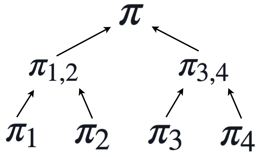
To keep the guarantee of soundness, we can bound in advance the number of steps of recursion we perform. Above we mentioned that our PCD scheme can also be modified to work for vectors of proof inputs. Instead of performing recursion in a linear inductive fashion, we can instead perform it on trees of proofs.
One option would be to construct a binary tree of proofs with a bounded depth $d$. Here each proof attests to the correctness of all proofs in the tree it descends from.
Another option is to simply ignore the issue, as so far this is only theoretical and no concrete attacks have been demonstrated. Intuitively it feels as though soundness of even unbounded recursion should reduce to soundness of the underlying proof system. Caveat emptor.
Recent Results and Future Work
Note that in developing a scheme for recursive composition we have devised a technique for producing a single proof for an NP relation in which the components of the relation are performed by circuits paramaterized by different cryptographic primitives, here elliptic curves. We might ask if this can be generalized, and the answer is yes.
One such generalization has triggered interest in generating a lollipop of curves. We have already observed that the MNT curves are inefficient, but so far are necessary for pairing-friendly recursive composition. We can partly solve this issue by introducing a third and more efficient “stick” curve connected to the two cycle curves. The majority of computation is done in the stick, with a proof fed into the main cycle curve along with the $n-1$th inductive proof, producing a wrapper proof to be fed into the second curve in the cycle to produce the $n$th inductive proof.
We may not even be interested in recursive composition at all, but rather in composition of restricted depth. Instead of using a cycle of curves, here we want to create a chain of curves. In the case of a 2-chain, we want curves $G_1, G_2$ such that if $|G_2| = r$, $G_1$ is defined over a base field $\mathbb{F}_r$ of size $r$. This allows for operations in the first curve $G_1$ to be efficiently computed in the circuit which $G_2$ paramaterizes. This can be used, for example, for the verification of BLS signatures inside of a circuit, useful because of their ability to be aggregated or used for $n$-of-$m$ threshold signatures. This depth-2 style of composition has recently been used by Zexe with curve BLS12_377; such curves can be generated via the Cocks-Pinch method.
Another possible technique would be to eliminate the use of elliptic curves altogether in the proof system used. This is the approach taken by Fractal, by developing and using a proof system which is instantiated only with a field $\mathbb{F}$ and a cryptographic hash $H$. This counter-intuitively achieves quantum security not by adding assumptions, but by removing them. Since we know quantum-resistant hashes exist, we know that this scheme can be instantiated to be secure against a quantum adversary. However, proof sizes are currently quite large at around 80-200kB.
Finally, Halo is a recently developed proof system which aims to improve the efficiency of recursion by using elliptic curve cycles which do not leverage pairings, in a manner which also eliminates having a trusted setup by using a non-preprocessing proof system. This is similar to Bulletproofs, in that the lack of setup prevents us from creating a succinct cryptographic description of our circuit. We are rather guaranteed that the verifier will need to read in the entire circuit, with a linear verificaiton runtime of $O(n)$ where $n$ is the circuit size. This is instantiated in Halo by a final multi-exponentiation in verification.
Resources and Further Reading
Alessandro Chiesa’s original work on Proof Carrying Data is the basis for the above construction.
The bulk of theory for recursive composition of proofs can be found in Recursive Composition and Bootstrapping for SNARKs and Proof-Carrying Data by Nir Bitansky, Ran Canetti, Alessandro Chiesa, and Eran Tromer.
The first implementation of recursive proofs was achieved in Scalable Zero Knowledge via Cycles of Elliptic Curves by Eli Ben-Sasson, Alessandro Chiesa, Eran Tromer, and Madars Virza. The majority of the exposition in this post was adapted from this paper, which is well-worth reading for additional depth.
The impossibility results for cycles of elliptic curves were taken from On cycles of pairing-friendly elliptic curves by Alessandro Chiesa, Lynn Chua, and Matthew Weidner.
Thanks
I am at least mildly indebted to Alessandro Chiesa for discussions about proof system reductions, and Dev Ojha for help understanding Fractal. I am also grateful to Eli Ben-Sasson and Ariel Gabizon for clarifications regarding STARKs on twitter.
I would also like to thank Kobi Gurkan, Georgios Konstantopoulos, and Alan Flores-Lopez for comments and critical feedback.